Natural Computing Lecture, March 8th, 2022

The Cellular Potts Model

A complex cellular automaton for modelling tissues

Inge Wortel
inge.wortel@ru.nl
Data Science, RU

Before we start

Master Open Day:

March 10^th, 19:30-20:15 (online)
Students for Q&A

Last week: cellular automata

CAs:

a grid with states (a few or many)...
...which change according to rules (deterministic/stochastic)
Typically, these rules are local, but global patterns may emerge.

This week: cellular Potts models (CPMs), a more complex CA.

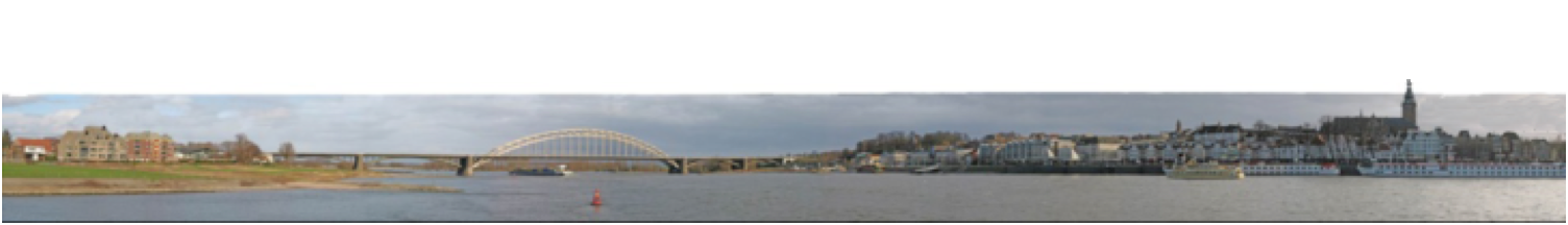
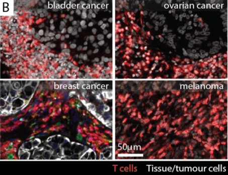
For example: simulating T-cell infiltration into a tumour

Question

What difference(s) do you see with the models from last week?

Question
What difference(s) do you see with the models from last week?

Cellular Potts Model (CPM) history: the cell sorting mystery

In the 1990s, biologists had:

observed that when mixing two types of embryonic cells, they spontaneously sort themselves
hypothesized that this was due to a difference in adhesion between the two cell types

...But how could they prove that this explanation was sufficient?

$\rightarrow$ Graner & Glazier wanted to build a computer model as proof of concept.

Starting point: the Ising model/Potts model

The following model already existed, describing how magnetic spins self-align:

The Potts model

The Potts model is a graph (grid) ${\cal G}=(\mathbf{V},\mathbf{E})$ with node identities $\sigma_\mathbf{V}$ and an associated adhesion energy function $$ {\cal H} = J \sum_{ \{i,j\} \in \mathbf{E}} \delta ( \sigma_i, \sigma_j ) \ . $$


${\cal H}=32J$	${\cal H}=20J$

The system tends to minimize this adhesion energy function; i.e.: to keep the same states together so as to minimize this "surface energy".

Stochastic simulation of Potts models

Metropolis-Algorithm:
Randomly choose a source and a neigbouring target. Copy "source" to "target" state with probability $$P(\Delta{\cal H},T) = \begin{cases} 1 & \Delta{\cal H} < 0, \\ e^{-\Delta{\cal H}/T} & \text{else.} \end{cases}$$

$P=1$

$P=e^{-6J/T}$

A simulation now consists of a series of such copy attempts. We define a Monte Carlo step as the number of copy attempts equal to the number of pixels on the grid.

Question

How does this compare to the CAs discussed last week?

Question
How does this compare to the CAs discussed last week?

The temperature T

What are we still missing?

For the cell sorting problems, we don't just have two spin states (/cell types), but also individual cells. These cells can move but they cannot just disappear.

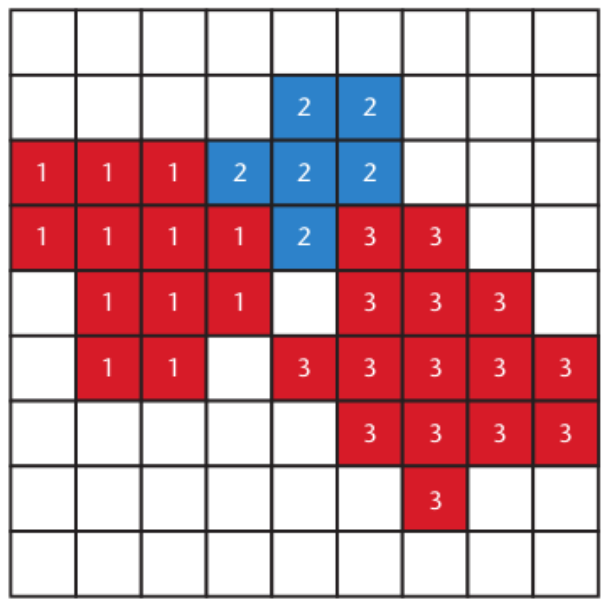
Graner and Glazier: the Cellular Potts Model (CPM)

A grid containing pixels of different identities
Multiple pixels of the same identity form a cell (= level 1 "state")
Mutiple identities can be treated as the same cell type (= level 2 "state")

Cickovski et al.
doi: 10.1109/MCSE.2007.74

The cellular Potts model: cells and cell types

Elements with the same identity $\sigma$ form a cell. The surface energy $J$ between cells now depends on the cell type $\tau$:

$$ {\cal H} = \sum_{(i,j)} \color{red}{J_{\tau_i,\tau_j}} \delta ( \sigma_i, \sigma_j ) $$

The cellular Potts model: cells and cell types

Elements with the same identity $\sigma$ form a cell. The surface energy $J$ between cells now depends on the cell type $\tau$. We also introduce a volume term

$$ {\cal H} = \sum_{(i,j)} J_{\tau_i,\tau_j} \delta ( \sigma_i, \sigma_j ) + \color{red}{\sum_{\sigma}\lambda_\tau ( |\{i \mid \sigma_i=\sigma\}|-v_\tau )^2} $$

We can obtain cells of different sizes that don't simply disappear:

Question

Beyond the addition of cells and cell types, what has changed fundamentally compared to the CAs discussed last week?

Question
Beyond the addition of cells and cell types, what has changed fundamentally compared to the CAs discussed last week?

Graner & Glazier, Phys Rev Lett 1992

The CPM as a model formalism

Graner and Glazier's "CPM" provided proof of concept for the cell sorting problem. But it would prove (much!) more powerful than that:

CPMs exhibit volume exclusion: each pixel can only belong to one cell at one time.
Thus, cells naturally interact with each other: to move, they automatically push others away.
Such interactions emerge from underlying (local) dynamics; we don't have to impose any forces.
Cell behavior and shape naturally arises from these interactions...
...and we can easily extend the model by adding anything we want to the Hamiltonian!

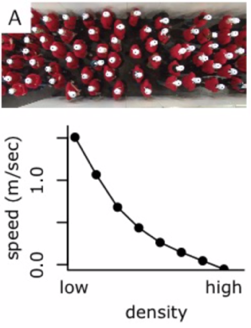
Our research: traffic jams in the body

Crowd dynamics

Garcimartin et al., Transportation Research Procedia (2014)
Pastor et al., Physical Review E (2015)

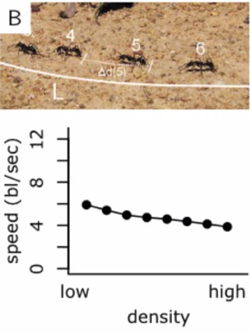
Crowd dynamics in nature

How do T cells behave compared to humans or ants?

Migration: The Act model

Cells move if we add positive feedback on protrusive activity ($\approx$ actin polymerization)¹:

Parameters:
λ_Act	$\approx$	protrusive force
Max_Act	$\approx$	polymerized actin lifetime
¹Niculescu et al. PLoS Computational Biology, 2015.

Max_Act

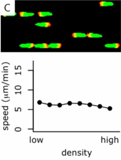
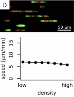
Simulating T cell one-lane traffic

Are T cells like ants?

Model prediction: T cells seem to behave more like ants!

Crowd dynamics

Jeremy Postat & Judith Mandl, McGill University

Verification in the lab

Summary

The cellular Potts model is a cellular automaton with a stochastic, asynchronous update rule.

The cellular Potts model can be adapted to different biological scenarios by adding terms to its Hamiltonian function.

In the assignment, you will implement your own cellular Potts simulation using a framework developed by us (or you can make your own)!

After the break, Shabaz Sultan will talk about implementing large-scale cellular Potts simulations on GPUs.